


Abstract
Copy number variants (CNVs) are currently defined as genomic sequences that are polymorphic in copy number and range in length from 1000 to several million base pairs. Among current array-based CNV detection platforms, long-oligonucleotide arrays promise the highest resolution. However, the performance of currently available analytical tools suffers when applied to these data because of the lower signal:noise ratio inherent in oligonucleotide-based hybridization assays. We have developed wuHMM, an algorithm for mapping CNVs from array comparative genomic hybridization (aCGH) platforms comprised of 385 000 to more than 3 million probes. wuHMM is unique in that it can utilize sequence divergence information to reduce the false positive rate (FPR). We apply wuHMM to 385K-aCGH, 2.1M-aCGH and 3.1M-aCGH experiments comparing the 129X1/SvJ and C57BL/6J inbred mouse genomes. We assess wuHMM's performance on the 385K platform by comparison to the higher resolution platforms and we independently validate 10 CNVs. The method requires no training data and is robust with respect to changes in algorithm parameters. At a FPR of <10%, the algorithm can detect CNVs with five probes on the 385K platform and three on the 2.1M and 3.1M platforms, resulting in effective resolutions of 24 kb, 2–5 kb and 1 kb, respectively.
INTRODUCTION
DNA copy number variation comprises a significant component of total genetic variation in human ( 1–4 ), chimpanzee ( 5 ) and mouse ( 6–9 ) populations. CNVs have been associated with disease susceptibility ( 10–16 ) and underlie variation in gene expression ( 17 ). To date, the genome-wide discovery of CNVs has been limited to large (>20 kb) events due to technological constraints. In order to accurately assess the impact of copy number variation on phenotype, as well as to learn more about their fine structure and origins, we must first be able to reliably detect CNVs of all sizes and accurately determine their genomic boundaries.
The most common genome-wide approaches to identify CNVs are array-based. These platforms include bacterial artificial chromosome (BAC) array comparative genomic hybridization (aCGH) ( 18 , 19 ), long oligonucleotide arrays ( 20–22 ) and single nucleotide polymorphism (SNP) genotyping arrays ( 23 ). A critical aspect in selecting a platform for CNV detection is effective resolution, which we define as the length of the shortest CNV that is detectable at an acceptable false positive rate (FPR). A number of factors contribute to resolution, including probe density (i.e. the number of probes that interrogate a region of the genome), probe specificity and sensitivity. Due to their high-probe density, long oligonucleotide arrays theoretically have the highest resolution and genome coverage of the three platforms ( 24 , 25 ). However, the higher level of noise of these platforms ( 24 , 26 ) has hampered efforts to mine these data for novel CNVs using available analytical tools, which were designed for BAC-array analysis. To date, there has been only one published account of a method designed specifically for detecting CNVs from such data ( 27 ), but there has been no comprehensive analysis of the achievable genome-wide resolution of these platforms.
The goal of our work was to develop a method for detecting CNVs specifically from long-oligo aCGH data, characterize its sensitivity, FPR and effective resolution and compare it to other CNV detection algorithms. Our focus is the detection of homozygous changes in the inbred mouse genome. Detection of heterozygous germline changes or somatic changes in mixed cellular populations may present additional challenges due to diminished signal intensity. However, existing computational tools detect even homozygous CNVs with relatively low sensitivity and unacceptably high FPRs. Although sequence divergence between a probe and its target impacts hybridization, no existing CNV detection algorithm has addressed this problem in the context of oligo-aCGH. Here, we show that there is a strong association between regions of sequence divergence and hybridization signal in high resolution aCGH data from inbred strains of mice. We present a method that optionally incorporates sequence information into a Hidden Markov Model (HMM)-based calling algorithm. We assess its sensitivity and precision, and compare its performance to other algorithms, three of which are commonly used for lower resolution platforms and one recently developed for dense microarrays.
MATERIALS AND METHODS
Sample preparation and array comparative genomic hybridization
DNA was extracted from the spleens and kidneys of healthy, young adult (age 8–12 week) 129X1/SvJ and C57BL/6J mice (The Jackson Laboratory, Bar Harbor, ME, USA). Different DNA samples were used for each aCGH platform (385K, 2.1M and 3.1M). The aCGH studies were performed using long oligonucleotide arrays designed and manufactured by Roche NimbleGen (Madison, WI, USA). The aCGH experiments were performed using a single array (385K-aCGH) with a median probe spacing of 5.2 Kb (MM6, NCBI Build 34), a single array (2.1M-aCGH) with a median probe spacing of 1.015 Kb (MM8, NCBI Build 36) or an 8-array set (3.1M-aCGH) with median probe spacing of 0.49 Kb (MM7, NCBI Build 35). Labeling, hybridization, washing and array imaging were performed as previously described ( 9 , 22 ). All mouse genome coordinates are based on NCBI Build 36 (MM8). Roche NimbleGen probe coordinates were re-mapped using liftOver ( http://genome.ucsc.edu/cgi-bin/hgLiftOver ). Data are available at GEO ( http://www.ncbi.nlm.nih.gov/geo/index.cgi ) under accession GSE10511.
Algorithm overview
We developed Washington University HMM (wuHMM) specifically to maximize CNV detection on high density, long oligonucleotide arrays. wuHMM is comprised of several stages: clustering log2-ratios, finding regions more likely to contain CNVs, performing local CNV segmentation and scoring ( Figure 1 A). The clustering stage bins log2-ratios for input to the HMM, which facilitates the incorporation of sequence information. There is an optional stage in which each chromosome is partitioned according to sequence divergence between the probe and target genomes based on independently derived genotype data. Segmentation is achieved by first searching for seeds consisting of short runs of probes with large magnitude log2-ratios. Seeded regions are then input to an HMM for segment boundary detection and scoring. The HMM ( Figure 1 B) is comprised of five states that represent normal and abnormal DNA copy number. The model requires a minimum length of stay in abnormal states in order to prevent singleton outliers from being called as CNVs. CNVs are scored based on log2-ratio magnitude, number of probes and local noise.
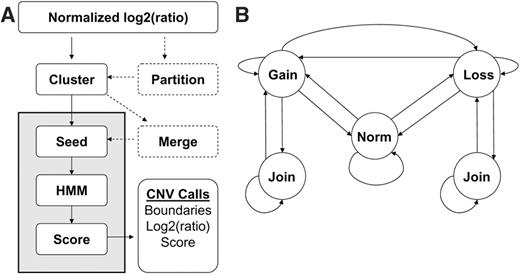
( A ) Flow diagram of the wuHMM algorithm. Dashed processes are optional and are executed when the sequence divergence information is utilized. Processes in gray were repeated on permuted probe locations to generate null score distributions for each chromosome. ( B ) Hidden Markov Model. ‘Norm’, ‘Gain’ and ‘Loss’ indicate states representing normal, increased, and reduced DNA copy number, respectively. Not shown, but implemented, are multiple states per abnormal state that enforce a minimum number of probes per abnormal state. This minimum is automatically selected for each seeded region as described in the Methods section. Transitions are permitted between normal, increased and reduced states. A ‘Join’ state can transition to itself or back to the corresponding abnormal state.
wuHMM can be downloaded from: http://groups.google.com/group/wuhmm . Default parameters (seed length, number of clusters and noise penalty) are set to optimized values based on the sensitivity and FPR of wuHMM applied to data of known copy number. These parameters and the use of sequence divergence data can be specified by the user.
Sequence divergence
In this optional pre-processing step, partitioning of a chromosome is accomplished by utilizing a three-state HMM, in which the states represent regions of sequence divergence or similarity compared to a reference genome or runs of no genotype calls ( Supplementary Figure 1 ). The reference is the C57BL/6J inbred mouse genome. The observations in the model are determined by the genotypes of 138 608 known SNPs ( 28 , 29 ). Specifically, an observation is coded as ‘0’ when the genotype differs between the test and reference genomes, as a ‘1’ when the genotypes agree, and ‘n’ when there is no call in either strain. This model is appropriate for pair-wise comparisons between inbred mouse strains containing genomic regions of high pair-wise polymorphism rates. We required that the system remain within a state for at least five observations, yielding an average minimum block size of 87 kb, which lies within the estimated size range of ancestral block sizes in inbred mice (mean: 58 kb, range:1 kb to 3 Mb) ( 30 ). The HMM is trained by expectation maximization.
Clustering
We clustered probes by log2-ratios to achieve two aims. First, clustering facilitated the normalization of log2-ratios between regions of sequence divergence and similarity. Second, binning probes by log2-ratios provided a convenient means of linking the decoded states of probes, as determined by the HMM, to biologically meaningful DNA copy number states (normal, gain or loss). The following procedure assigned cluster labels to each probe, ensuring that there is the expected number of clusters for input to the HMM: We used partitioning among medoids (PAM), as implemented in R's ‘cluster’ package using the clara function ( 31 ). When sequence divergence information is utilized, probes are separated according to sequence divergence state first, then clustered and labeled as described earlier ( Supplementary Figure 2 ). Probe cluster labels are treated as observations by the HMM.
Divide probes in two groups:
Group A: probes with log2-ratios ≥0
Group B: all other probes
Cluster probes in each group into floor( n /2) + 1 groups, where, n = number of clusters.
Merge the cluster in Group A having the minimum magnitude mean log2-ratio and the cluster in Group B with the minimum magnitude mean log2-ratio into one cluster, resulting in n clusters.
Rank clusters by mean log2-ratio.
Label each probe by the rank of its cluster.
Seeding
It was necessary to target regions of the genome that were likely to contain CNVs prior to executing a more sensitive CNV-detection algorithm. Without the seeding step we found that training the HMM on whole chromosomes periodically led to reduced power to detect short CNVs and misclassification of large regions of chromosomes as CNVs. We identified regions likely to harbor CNVs by the presence of consecutive probes with large magnitude log2-ratios. This was achieved using a stringent HMM in which the emissions from abnormal states were restricted to corresponding clusters. We trained the stringent HMM and performed decoding on each chromosome separately, producing a set of seeds. A seeded region, which was used as input to the more sensitive CNV detection algorithm, was defined as the seed-spanning region plus 100 probes on either side. Overlapping seeded regions were merged.
Hidden Markov Model
Our HMM generally follows the approach to decoding copy number from aCGH data as first described by Fridyland et al. ( 32 ) with several notable exceptions. The true, unobserved DNA copy number of a given probe is treated as a hidden state and probe cluster labels are the observed emissions from the model ( Figure 1 B). The initial emissions of abnormal states are weighted most heavily to the highest and lowest cluster ranks. Emissions from abnormal states cannot be from clusters with oppositely signed means. The initial transition probabilities are set such that most of the chromosome is assumed to be in a normal state. ‘Joiner’ states, which have an initial emission distribution weighted toward the corresponding abnormal state but permit emissions from all states, exist in order to prevent CNV call fragmentation. Final emission and transition probabilities are determined by the Baum and Welch expectation maximization algorithm for each seeded region until convergence of the model likelihood, which is typically achieved in fewer than 10 iterations. Training is repeated for each seeded region, varying the minimum length of stay in an abnormal state from 3 to 10. The model with the greatest likelihood is then used to determine copy number with the Viterbi decoding algorithm ( 33 ). The GHMM library ( http://ghmm.sourceforge.net/software ) was used to implement the HMMs.
Scoring function and permutation

n = number of probes comprising the CNV
cnv_nps = index probes within a distance of 5 × length of the call that share the same sign as the mean (log2-ratio) cnv
W = noise weight term.
In attempting to determine the significance of a CNV score, probe locations were randomized for each chromosome, the segmentation method was applied, and the best score was stored. We repeated these steps 100 times to generate a null distribution of CNV scores for each chromosome. P -values were computed using R's ‘quantile’ function, which uses linear interpolation to estimate the given quantile ( 34 ).
Validation
Two methods were used to validate CNV calls. First, we used replicate aCGH experiments at increasing probe density to identify probes on the 385K array that have reproducible log2-ratio shifts. This information was used to assess the performance of wuHMM and other CNV detection algorithms, as described subsequently (see Sensitivity and false positive rate section). We performed three replicate aCGH experiments at increasing probe densities: two 2.1M-aCGH (each comprised of a single 2.1M feature array) experiments and one 3.1M-aCGH (eight-385K arrays) experiment. We included probes for assessment analysis only if there were at least four probes in the 6 kb centered at a 385K probe (median inter-probe distance on the 385K array is 6 kb) on both the 2.1M and 3.1M platforms. We termed these ‘informative probes’. The gold standard is the copy number status (i.e. gain, loss, or neutral) of the informative probes. The copy number status of an informative probe was defined according to the |mean log2-ratio region | on the replicate arrays. Specifically, an informative probe was considered to represent a DNA copy number change if the |mean log2-ratio region | > threshold on all replicates, where the threshold varied between arrays and regions of sequence similarity and divergence. If an informative probe was in a divergent region and its log2-ratio < 0, then it was considered to represent a DNA copy number change if |mean log2-ratio region | > SD divergent_blocks for all replicate arrays, where SD divergent_blocks is the standard deviation of probes in divergent regions. For all other informative probes, the threshold is the standard deviation of the sequence similar regions. The SD cutoffs for the similar regions were 0.2416, 0.2176 and 0.2200 for the 385K, 2.1M and 3.1M platforms, respectively. SD cutoffs for the divergent regions were 0.4115, 0.3457 and 0.3142.
Independent validation of 10 CNVs (all deletions) was achieved by attempting to amplify by PCR regions within CNV boundaries. PCR primers ( Supplementary Table 1 ) were designed to localize within a CNV. Amplification reactions contained 10 μl of Jumpstart Ready Mix Taq (Sigma, http://www.sigmaaldrich.com ), 100 ng of each primer and 10 ng of genomic DNA in a final volume of 20 μl. Amplifications were performed on a PTC-225 Peltier Thermal Cycler (MJ Research, Waltham, Massachusetts) at standard conditions for 30 cycles and the product was run on a 2% agarose gel, stained with ethidium bromide and visualized on a GelDoc (BioRad, Hercules, California).
Sensitivity and false positive rate
We calculated sensitivity and FPR of CNV detection algorithms on the 385K platform based on the gold standard. We calculated the sensitivity of CNV calls as the number of probes representing a true copy number change within predicted CNVs divided by the total number of probes representing true copy number changes in the gold standard. We defined the FPR as one minus the proportion of CNVs that are significantly enriched for probes representing a true copy number change. The enrichment of a CNV was determined by randomly selecting equally sized regions of the chromosome and recording the proportion of probes representing true copy number changes that they contain. We repeated this step 100 times, generating a null distribution of enrichment values. We designated an observed call as a true positive if its enrichment value exceeded 95% of the random enrichment values. We observed that due to differences in probe design between platforms, some high-scoring calls on the 385K-aCGH were not sufficiently covered on the higher resolution platforms. Therefore, we excluded calls that were comprised of fewer than 25% informative probes in any performance analysis for wuHMM and other segmentation algorithms. Also, singletons and doubleton calls were not considered in any performance analysis.
Other segmentation algorithms
We applied GLAD ( 35 ), CBS ( 36 ) and BioHMM ( 37 ) to the 385K-aCGH data using BioConductor's snapCGH package ( 38 ). To reduce the amount of processing time required by GLAD and DNACopy, we divided each chromosome into blocks of ∼50 Mb. These methods do not explicitly define segments as amplified or deleted. Segments were classified as ‘abnormal’, if the predicted log2-ratio was >0.35 or <−0.35. We used BreakPtr ( 27 ) version 1.0.5 downloaded from http://tiling.mbb.yale.edu/BreakPtr/ . We trained BreakPtr using known gains and losses in 129X1/SvJ. We used the Finder-Core module with the default transition probabilities.
Other statistical tests
To test the association between sequence divergence and signal intensity, probes were partitioned according to sequence divergence state as described. A t -test, using R's t.test function not assuming equal variances, was applied to the raw, linear-scale signal intensities of the129X1/SvJ channel.
RESULTS
Sequence divergence affects probe hybridization signal
There are long regions of the 129X1/SvJ aCGH data that exhibit a dispersed but pronounced negative log2-ratio ( Figure 2 ). These regions differ from true deletions, which are comprised almost entirely of negative log2-ratios. It was previously hypothesized that a similar phenomenon observed in BAC arrays was a result of decreased hybridization efficiency due to sequence polymorphism between the test and reference genomes ( 8 ). There are regions of classical inbred mouse genomes that exhibit pair-wise polymorphism rates exceeding 1/400 base pairs, reflecting divergent subspecies ancestry ( 30 ). We tested the hypothesis that the regions of dispersed negative log2-ratios represent blocks of different ancestry in C57BL/6J versus 129X1/SvJ by partitioning the 129X1/SvJ genome into blocks of sequence similarity and divergence relative to the C57BL/6J sequence using ∼140 000 genotype calls. We found 1826 sequence-similar blocks and 1790 sequence-divergent blocks (median length 190 and 262 kb, respectively). As predicted, the signal intensity of 129X1/SvJ in regions of sequence divergence is significantly lower than in regions of sequence similarity in all experiments in the majority (18/19, 17/19 and 13/19, on 385K, 2.1M, and 3.1M arrays, respectively) of autosomes ( Table 1 ). Similarly, the test channel intensity is lower in divergent blocks of 385K-aCGH data from 18 other inbred mouse strains, suggesting that the association between blocks of sequence divergence and aCGH signal is not an idiosyncrasy of a single strain comparison but represents a general phenomenon (data not shown). In order to determine the impact of sequence divergence on segmentation algorithms, we attempted to validate by PCR five deletions in divergent regions called by a variety of algorithms on 385K-aCGH data. All five putative deletions failed to validate ( Supplementary Figure 3 and data not shown), indicating that they do not represent true deletions but are instead artifacts of sequence polymorphism affecting hybridization. This underscores the importance of incorporating methods to differentiate between CNVs and blocks of high polymorphism rates in order to reduce the number of false positive segment calls.
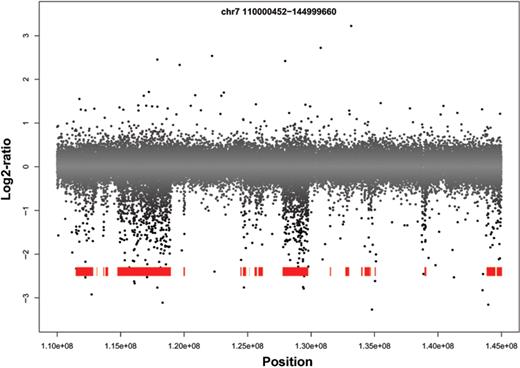
3.1M-aCGH log2-ratio plot of 129X1/SvJ chromosome 7. Blocks of sequence divergence are shown in red. Blocks of divergence correspond to aCGH probes with lower log2-ratios and can potentially confound CNV calling algorithms.
Relationship between sequence identity and aCGH signal
| Chr | 385K-aCGH | 2.1M-aCGH | 3.1M-aCGH | ||||||||||||
|---|---|---|---|---|---|---|---|---|---|---|---|---|---|---|---|
| Probe count | Test signal | Probe count | Test signal | Probe count | Test signal | ||||||||||
| M | MM | M | MM | P -value | M | MM | M | MM | P -value | M | MM | M | MM | P -value | |
| 1 | 13 188 | 16 205 | 4655 | 4489 | 8.90E-15 | 72 049 | 91 734 | 3550 | 3331 | 1.56E-82 | 101 963 | 124 620 | 3266 | 3120 | 2.60E-44 |
| 2 | 13 909 | 13 990 | 4612 | 4455 | 1.30E-12 | 76 513 | 77 565 | 3516 | 3463 | 5.04E-06 | 111 127 | 114 313 | 2999 | 2854 | 2.80E-48 |
| 3 | 11 306 | 11 954 | 4682 | 4485 | 7.70E-16 | 64 400 | 67 515 | 3427 | 3316 | 9.24E-20 | 85 703 | 90 427 | 2494 | 2422 | 2.00E-12 |
| 4 | 8747 | 13 700 | 4628 | 4434 | 4.00E-15 | 48 344 | 78 238 | 3612 | 3351 | 3.07E-81 | 72 101 | 111 243 | 2508 | 2427 | 4.50E-16 |
| 5 | 9935 | 12 574 | 4646 | 4505 | 1.20E-07 | 55 891 | 69 525 | 3601 | 3497 | 2.35E-14 | 79 773 | 102 559 | 2703 | 2629 | 1.70E-15 |
| 6 | 12 095 | 10 437 | 4661 | 4414 | 1.60E-27 | 67 247 | 57 338 | 3205 | 3113 | 1.49E-14 | 94 546 | 82 567 | 2865 | 2772 | 3.20E-19 |
| 7 | 8542 | 11 126 | 4626 | 4359 | 8.40E-21 | 48 250 | 63 624 | 3334 | 3029 | 6.48E-116 | 74 732 | 93 915 | 3606 | 3450 | 1.60E-21 |
| 8 | 7962 | 11 620 | 4662 | 4379 | 2.40E-23 | 43 465 | 65 059 | 3303 | 2986 | 3.81E-124 | 65 419 | 94 888 | 3646 | 3422 | 1.20E-39 |
| 9 | 7903 | 11 389 | 4617 | 4422 | 2.20E-14 | 43 317 | 62 739 | 3295 | 3137 | 9.58E-32 | 65 014 | 94 193 | 2385 | 2095 | 7.00E-149 |
| 10 | 13 865 | 5 569 | 4670 | 4562 | 2.10E-04 | 77 515 | 32 036 | 3139 | 3183 | 1.49E-03 | 106 880 | 43 868 | 2011 | 2000 | 2.60E-01 |
| 11 | 11 058 | 8255 | 4567 | 4438 | 5.40E-06 | 62 019 | 44 518 | 3311 | 3210 | 3.13E-13 | 95 181 | 69 851 | 2445 | 2453 | 5.00E-01 |
| 12 | 8686 | 7689 | 4660 | 4417 | 1.60E-17 | 50 261 | 43 365 | 3057 | 2972 | 6.60E-10 | 69 487 | 61 473 | 3193 | 3220 | 1.60E-01 |
| 13 | 9250 | 8121 | 4671 | 4507 | 2.60E-08 | 51 745 | 45 216 | 3062 | 2916 | 7.69E-28 | 75 538 | 63 704 | 3269 | 3193 | 8.30E-06 |
| 14 | 7982 | 9259 | 4682 | 4389 | 4.90E-23 | 46 043 | 51 318 | 2918 | 2820 | 2.87E-13 | 60 075 | 73 647 | 2674 | 2683 | 5.10E-01 |
| 15 | 7888 | 7931 | 4637 | 4388 | 4.60E-16 | 43 200 | 43 898 | 3073 | 2814 | 1.34E-71 | 63 517 | 62 254 | 2512 | 2365 | 1.90E-42 |
| 16 | 7768 | 6861 | 4616 | 4563 | 7.70E-02 | 44 036 | 37 931 | 2967 | 2856 | 4.09E-15 | 60 921 | 51 324 | 2474 | 2465 | 4.20E-01 |
| 17 | 5464 | 8188 | 4642 | 4486 | 1.10E-05 | 30 042 | 46 894 | 3025 | 2958 | 1.72E-05 | 42 824 | 67 144 | 2851 | 2708 | 1.80E-23 |
| 18 | 6324 | 7615 | 4707 | 4538 | 4.80E-08 | 34 739 | 41 374 | 2999 | 2980 | 1.93E-01 | 48 748 | 60 966 | 3124 | 3053 | 9.70E-07 |
| 19 | 7336 | 1773 | 4645 | 4490 | 1.10E-03 | 40 292 | 9748 | 3111 | 3008 | 2.57E-05 | 60 703 | 14 985 | 3078 | 3055 | 3.20E-01 |
MM, regions of high polymorphism between C57BL/6J and 129X1/SvJ (‘mismatched’); M, non-polymorphic regions (‘matched’). Probe count columns contain the number of probes within M and MM regions. Test signal columns contain the mean, single channel, linear-scale aCGH intensities of the M and MM regions. The P -value is the result of a t -test, testing the difference of the mean signals of M and MM probes, as described in the Methods section.
Gold standard
In order to assess the FPR and sensitivity of wuHMM and other segmentation methods, we needed to determine the true copy number state of each assayed region of the 129X1/SvJ genome. Replication by independent methods (e.g. PCR, qPCR and FISH) is the accepted standard by which CNV predictions are considered validated. It would not be practical to use any of these methods to systematically validate the thousands of predictions made by all algorithms tested. Instead, we determined the 129X1/SvJ copy number of the 6 kb region spanning each 385K-aCGH probe (approximately equal to the median spacing of the platform) by comparison to replicate experiments at higher resolutions (two 2.1M-aCGH, one 3.1M-aCGH). We reasoned that if the signal from a 385K-aCGH probe represents a true copy number change, then the log2-ratio shift will be reproducible on higher density platforms with more probes reflecting the variation. The higher density platforms contain, on average, 5.6 and 8.7 probes per 6 kb window on the 2.1M and 3.1M platforms, respectively. 336 470 probes on the 385K array are informative (i.e. there were at least four probes in the 6 kb region spanning the probe on both the 2.1M and 3.1M platforms). Of the informative probes, we found that 1886 represented true copy number changes since they had reproducible log2-ratio shifts on all three replicate arrays. 1226 informative probes were singletons (i.e. probes representing a copy number change that are adjacent to informative probes that do not represent true copy number change). Two hundred and fifty-two probes were doubletons, similarly defined as an adjacent pair of validated probes surrounded by informative probes not representing true copy number change.
We next asked if it would be feasible to detect singletons or doubletons using only log2-ratio thresholds. SD multipliers were used to identify probes as potential CNVs. Even when the SD multiplier threshold >5 was applied, 89% of the called probes were false positives and <5% of the called probes were true positives ( Table 2 ). These results demonstrate that attempting to detect singletons or doubletons from a single experiment will result in unsatisfactory sensitivity and FPR. For this reason, we removed singletons and doubletons from both the gold standard and CNV predictions prior to the calculation of sensitivity and FPR. Four hundred and eight probes representing true copy number changes remained after removing singletons and doubletons.
Detection of singletons and doubletons on 385K-aCGH
| SD multiplier | Singleton sensitivity | Doubleton sensitivity | FPR | Number of probes (percent of total) |
|---|---|---|---|---|
| 0.25 | 0.869 | 0.881 | 0.993 | 251 166 (74.6) |
| 0.50 | 0.742 | 0.782 | 0.992 | 176 851 (52.6) |
| 0.75 | 0.631 | 0.698 | 0.989 | 118 501 (35.2) |
| 1.00 | 0.553 | 0.631 | 0.985 | 77 423 (23) |
| 1.25 | 0.487 | 0.560 | 0.979 | 50 327 (15) |
| 1.50 | 0.431 | 0.496 | 0.971 | 33 049 (9.8) |
| 1.75 | 0.376 | 0.425 | 0.963 | 22 172 (6.6) |
| 2.00 | 0.336 | 0.381 | 0.953 | 15 630 (4.6) |
| 2.25 | 0.300 | 0.329 | 0.942 | 11 409 (3.4) |
| 2.50 | 0.259 | 0.298 | 0.933 | 8594 (2.6) |
| 2.75 | 0.234 | 0.282 | 0.923 | 6698 (2) |
| 3.00 | 0.206 | 0.214 | 0.916 | 5270 (1.6) |
| 3.25 | 0.177 | 0.183 | 0.910 | 4226 (1.3) |
| 3.50 | 0.152 | 0.159 | 0.905 | 3384 (1) |
| 3.75 | 0.127 | 0.139 | 0.902 | 2718 (0.8) |
| 4.00 | 0.108 | 0.115 | 0.896 | 2200 (0.7) |
| 4.25 | 0.090 | 0.091 | 0.894 | 1786 (0.5) |
| 4.50 | 0.074 | 0.079 | 0.888 | 1415 (0.4) |
| 4.75 | 0.064 | 0.052 | 0.885 | 1109 (0.3) |
| 5.00 | 0.048 | 0.040 | 0.891 | 906 (0.3) |
| 5.25 | 0.037 | 0.036 | 0.897 | 735 (0.2) |
| 5.50 | 0.031 | 0.016 | 0.898 | 598 (0.2) |
| 5.75 | 0.024 | 0.012 | 0.899 | 467 (0.1) |
| 6.00 | 0.020 | 0.008 | 0.903 | 393 (0.1) |
We calculated the sensitivity and FPR of all CNV detection algorithms based on the 385K gold standard, which is defined as the copy number status of the informative probes. CNV predictions were considered correct if they contained a significantly enriched number of informative probes that represented a true copy number change. The FPR was calculated as one minus the ratio of the number of correct CNV predictions to the total number of CNV predictions. In this way, the FPR is presented at a CNV-level. However, the sensitivity could only be calculated at the level of individual probes because the total number of ‘correct’ CNVs remains unknown in our gold standard. The sensitivity is calculated as the ratio of the number of informative probes contained within predicted CNVs that represented a true copy number change to the total number of probes representing true copy number changes.
Scoring function
It is common practice to prioritize or rank CNV predictions for downstream analysis and experiments such as validation and evaluation of functional significance. We view this prioritization in terms of a scoring function that relates aspects of the call (e.g. the amplitude of deviation from a log2-ratio of 0, the number of probes within a segment) to the quality of the call. A well-designed scoring function will generate high scores for true positive calls and low scores for false positive calls. We first asked which choice of threshold acted as a better scoring function: the number of probes per segment, or the |mean log2-ratio| of the segment. We calculated the sensitivity and FPR of wuHMM across a range of parameter settings and reported the maximum sensitivity when the FPR was <15% ( Supplementary Table 2 and Supplementary Figure 4 ). The |mean log2-ratio| performed poorly (mean sensitivity = 8.5%). The number of probes per segment threshold performed substantially better (mean sensitivity = 40.6%), but we speculated that a scoring function that uses both parameters would provide further improvement. A combined scoring function (see Methods section) had the best performance at all parameter settings (mean sensitivity = 47.8%).
Next, we hypothesized that we could assign a statistical significance to CNV calls by generating a null distribution of scores for calls made on randomized data. On a per-chromosome basis, we randomized probe locations, executed wuHMM and stored the highest score. We repeated this process 100 times to generate a null distribution of scores. We calculated P -values for each observed call based on comparison of its score to the null distribution of scores. We found that the FPR of scores with P < 0.01 remained above 47%, indicating that this permutation approach to determining CNV call quality did not achieve an acceptable FPR. Therefore, the scoring function can be used to evaluate algorithm performance, but significance thresholds for the scores must be determined empirically.
Algorithm parameters
An important goal in developing wuHMM was to make it tunable such that changes in initial parameter settings would have predictable effects on performance and therefore could be adjusted to meet the needs of each individual analysis. We evaluated the effect of varying the number of clusters, the minimum number of probes required in the seeding stage, use of sequence information, and the scoring function noise penalty on wuHMM's sensitivity and FPR. First, we investigated the effect of varying only seed length and the number of clusters. We expected that increasing the seed length would decrease the overall sensitivity and FPR because larger values of the seed length would increase the likelihood that the algorithm would skip regions containing small CNVs. We executed wuHMM using a range of seed lengths and number of clusters, calculated the sensitivity and FPR at increasing score thresholds, and generated receiver operating curves ( Figure 3 ). As expected, we found that increasing the seed length reduced the maximum sensitivity (from 70% to 34%) and the maximum FPR (86–35%). The best performance (sensitivity = 53% at FPR < 10%) was achieved when seed length was 2, although a value of 3 performed nearly as well. There was no clear performance trend with increasing the number of clusters. The best performance (sensitivity = 50%, FPR < 10%), achieved with the number of clusters = 5, was substantially better than other numbers of clusters. These results demonstrate that seed length can be increased to decrease the maximum FPR at the expense of a much reduced sensitivity. Further, they show that a combination of seed length = 2 and number of clusters = 5 produces the optimal performance tradeoff. To determine if wuHMM would be generally applicable with these parameter settings (i.e. that it is not over-trained), we applied it to previously described data from 19 other inbred strains at the 385K resolution ( 9 ). Of the 72 previously discovered ‘high-confidence’ CNVs, 71 (98.6%) were detected with wuHMM using identical parameter settings (e.g. seed length = 2, number of clusters = 5, using sequence divergence information). Additionally, the range of call lengths and number of calls per genome are consistent with the 129X1/SvJ calls (length range: 9 kb to 4 Mb, median length = 138 kb, mean length = 460 kb). The calls per genome range from one (C57BL/6Tac) to 75 (Molf/EiJ) with a mean of 36 ± 17.
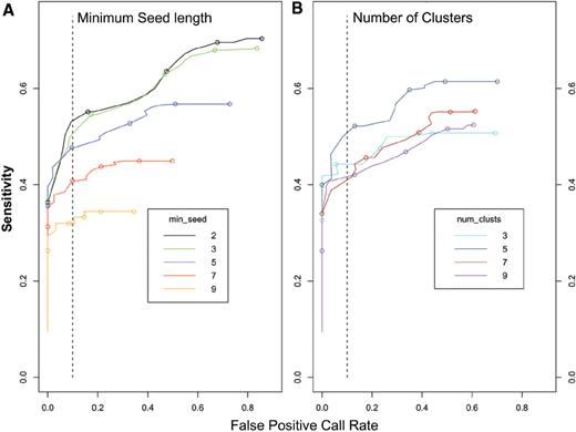
Receiver operating curves characterize the performance of wuHMM. ( A ) Each curve represents the performance of wuHMM at a given minimum seed length. Score cutoffs ranging from 0 to 2.5 were used to calculate sensitivities and false positive rates averaged across executions of wuHMM with different numbers of clusters. Circles represent score cutoffs of 0.0, 0.5, 1.0, 1.5 and 2.0, from right to left. The vertical dashed line represents a FPR = 10%. ( B ) The performance of wuHMM varying the number of clusters in the clustering stage. Score cutoffs ranging from 0 to 2.5 were used to calculate sensitivities and false positive rates averaged across executions of wuHMM with different seed lengths. As in (A), circles represent score cutoffs of 0.0, 0.5, 1.0, 1.5 and 2.0, from right to left, and the vertical dashed line represents a FPR = 10%.
We next analyzed the effect of incorporating sequence divergence on wuHMM's performance. We calculated the difference between the sensitivity and FPR of wuHMM with or without sequence divergence at increasing score thresholds. As predicted, utilizing sequence information reduced both the FPR and the probe-level sensitivity ( Figure 4 ). These effects were greatest for calls scoring between 0.8 and 1.4, a score range which includes validated gains and losses. We next calculated sensitivity and FPR using a range of values for the noise penalty, W, which decreases the score of calls in regions of greater noise (see Methods section). We found that increasing the noise penalty resulted in equalizing the FPRs between wuHMM with sequence information and without sequence information. At the same time, the sensitivity did not substantially improve, demonstrating that the use of a noise penalty with sequence divergence information results in worse overall performance.
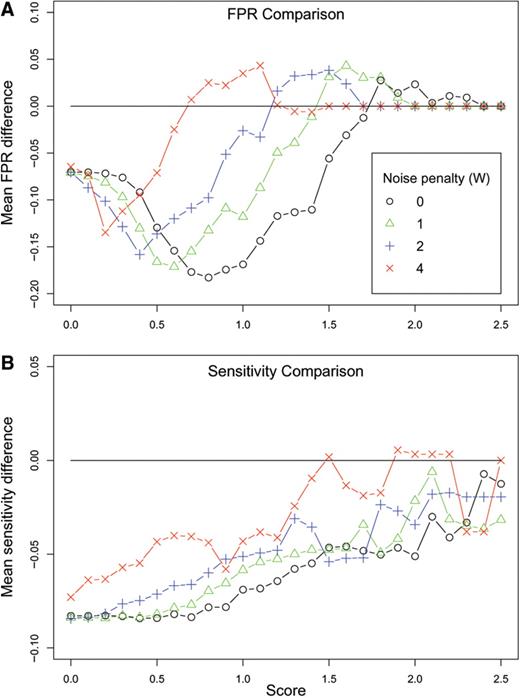
Performance differences between wuHMM with sequence divergence and without sequence divergence. ( A ) FPR difference. Y -axis is the difference between the average false positive rates at the given score cutoff. A value below the y = 0 line represents an improvement in the FPR when sequence divergence is utilized. ( B ) Sensitivity difference. Y -axis is the difference between the average sensitivities at the given score cutoff. In (A) and (B) each curve represents the performance difference with varying noise penalties (W). FPRs and sensitivities are averaged across a range of values for the number of clusters and minimum seed length.
Genotype information is not readily available for all aCGH experiments that may contain noise due to sequence divergence. We asked if using a noise penalty would improve FPR at an acceptable loss of sensitivity when sequence information is not available. We executed wuHMM without sequence information using a range of penalty values and calculated the sensitivity and FPR at increasing score thresholds ( Supplementary Figure 5 ). We found that there was no performance improvement when using any non-zero penalty. We concluded that for the range of values tested, the noise penalty does not enable the score function to differentiate between real calls and noise. Therefore, we recommend the use of conservative score thresholds when there is substantial noise in the data.
Effective resolution
Using parameter values that optimized sensitivity and FPR (seed length = 2, number of clusters = 5, noise penalty = 0), we applied wuHMM to all data sets. We selected a score threshold that yielded a FPR < 7% and sensitivity of 56% on the 385K platform. We attempted to independently validate 10 calls made from the 2.1M and 3.1M experiments by PCR. We considered a call to be validated when we were able to detect an amplified product in the C57BL/6J sample but not in the 129X1/SvJ sample. All 10 calls confirmed the wuHMM predictions, independently demonstrating that wuHMM can reliably detect calls comprised of as few as three probes on 2.1M-aCGH and seven probes on 3.1M-aCGH ( Figure 5 ).
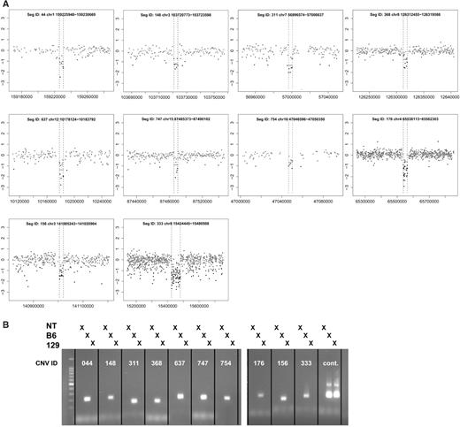
Validation of selected 3.1M-aCGH CNV calls in 129X1/SvJ. ( A ) Log2-ratio plots of validated 3.1M-aCGH CNV calls. The genomic position is plotted on the x -axis and the log2 (129X1/SvJ signal/C57BL/6J signal) is plotted on the y -axis. CNVs are annotated with a unique identifier (SegID) and boundaries. Dotted lines indicate CNV boundaries as determined by wuHMM. ( B ) PCR validation. All 10 deletions were validated by PCR, as demonstrated by a visible product using C57BL/6J, but not 129X1/SvJ genomic DNA. The marker is a 100 bp ladder. A region not deleted in 129X1/SvJ serves as a positive control. NT, no template.
We estimated the effective resolution of the 385K platform by determining the length of the call with the fewest probes with a score exceeding 1.9 (i.e. at a FPR < 7%) ( Table 3 ). Assuming that the relationship between CNV score and the FPR remains relatively constant across aCGH densities, we estimated the effective resolutions of the 2.1M and 3.1M platforms by averaging the lengths of the calls comprised of the fewest probes with scores exceeding 1.9 ( Table 3 ).
Effective resolution of aCGH platforms analyzed by wuHMM
| Platform | Resolution (kilobases) | SD | Segment length (base pairs) | Segment length (probes) | ||
|---|---|---|---|---|---|---|
| Platform | Resolution (kilobases) | SD | ||||
| Minimum | Median | Minimum | Median | |||
| 385K | 23.7 | 0.2629 | 23 577 | 191 594 | 5 | 23 |
| 2.1M-a a | 5.2 | 0.3336 | 1872 | 7618 | 3 | 7 |
| 2.1M-b b | 2.2 | 0.2846 | 1906 | 7067 | 3 | 7 |
| 3.1M | 1.1 | 0.2690 | 909 | 6156 | 3 | 9 |
a First technical replicate.
b Second technical replicate.
Comparison to other methods
We compared the performance of our approach to four other segmentation algorithms: Gain and Loss Analysis of DNA (GLAD), BioHMM, DNACopy, and BreakPtr. The performances of GLAD and DNACopy, as well as other HMM implementations have been compared previously using well-characterized BAC array and simulated data ( 39 , 40 ). Using default parameters, we applied each algorithm to the 385K-aCGH data, scored CNV calls, removed singletons, doubletons and calls comprised of <25% informative probes (see Methods section), and computed sensitivity and FPR based on the gold standard. In order to ensure an unbiased comparison of algorithms, we determined the lowest score cutoff at which each method reached a FPR <10%. For all methods this score threshold was 1.9. wuHMM reached the highest sensitivity, followed closely by DNACopy and more distantly by BreakPtr and GLAD ( Table 4 ). All HMM-based methods required less than an hour of execution time. Although input data was partitioned prior to input to DNACopy and GLAD, these methods still had the longest executions times at 1.4 and 12.4 h, respectively. BreakPtr appeared to be critically dependent on its training set. We initially trained the ‘no-change’ state with data from self-self hybridization, but this resulted in BreakPtr calling over 10% of the informative probes, resulting in a 99% FPR. Among currently available methods, wuHMM achieves the highest sensitivity while maintaining an acceptable FPR.
Performance of segmentation algorithms on 385K-aCGH data
| Method | Probe sensitivity (%) | Execution time (h) | Additional input |
|---|---|---|---|
| wuHMM | 56.1 | 0.17 | Genotype data |
| DNACopy | 54.4 | 1.4 | Partition input |
| BreakPtr | 43.9 | 0.02 | Supervised training |
| GLAD | 43.1 | 12.4 | Partition input |
| BioHMM | 21.6 | 0.1 | None |
| Method | Probe sensitivity (%) | Execution time (h) | Additional input |
|---|---|---|---|
| wuHMM | 56.1 | 0.17 | Genotype data |
| DNACopy | 54.4 | 1.4 | Partition input |
| BreakPtr | 43.9 | 0.02 | Supervised training |
| GLAD | 43.1 | 12.4 | Partition input |
| BioHMM | 21.6 | 0.1 | None |
DISCUSSION
Prior to this report, the selection of tools for the analysis of long oligonucleotide aCGH data was limited largely to software originally designed for other aCGH platforms, such as BAC-based or SNP genotyping arrays. We developed wuHMM to improve CNV detection from long oligonucleotide aCGH data that may be confounded by sequence divergence. wuHMM addresses sequence divergence by increasing the call stringency in sequence divergent regions of the genome. The effect of this strategy is to lower the FPR and, to a lesser extent, the sensitivity. In order to assess the algorithm, we developed a validated data set that should be a useful resource for the evaluation of other segmentation methods. By applying wuHMM to the validated data set, we demonstrated that it reaches the highest sensitivity among currently available methods at a FPR of <10%.
There are two caveats that apply to this analysis. First, in the current version of wuHMM, sequence divergent regions were estimated using only 140 000 SNPs. Therefore, small regions of sequence divergence may be missed. When more sequence data become available it can be incorporated into our method to better define the divergent regions, perhaps even down to the single aCGH probe level. Second, we expect that all existing CNV detection algorithms will exhibit reduced sensitivity when applied to aCGH data from outbred populations or samples with mixtures of somatic and germline copy number changes.
We estimate that effective resolutions of the 2.1M and 3.1M probe aCGH platforms, extrapolated based on a score threshold that yielded a FPR <10% on the 385K probe platform, are 2–5 kb and 1 kb, respectively. However, although we independently validated several CNVs shorter than 5 kb, the overall confidence in resolution estimates for the 2.1M and 3.1M probe arrays will require additional evaluation. The first genome-wide studies of normal copy number variation in the mouse genome, based on BAC-aCGH platforms, were limited to a resolution of ∼1 Mb ( 6–8 ). In 385K-aCGH data sets using a single whole-genome array (median probe spacing of 5.2 kb) and CNV analysis algorithms available at the time, we previously reported a total of five CNVs in the 129X1/SvJ genome ( 9 ). Applying wuHMM to the 385K-aCGH data, we can now detect 15 CNVs in the 129X1/SvJ genome at an empirical FPR <10%. Applying wuHMM to 3.1M-aCGH (an 8-fold increase in resolution) yields 167 CNVs. Theoretically, another 10-fold increase in probe density to a median probe spacing of ∼87 bases for the mouse genome will enable the resolution of ‘sub-CNV’ events (i.e. insertion–deletions). Comprehensive tools such as the ones presented here are necessary to accurately assess the phenotypic impact of CNVs, improve our understanding of CNV origins, and facilitate integrated quantitative trait locus (QTL) mapping, linkage and association studies.
ACKNOWLEDGEMENTS
Mice were kindly provided through a collaboration with the Mouse Phenome Project (The Jackson Laboratory, Bar Harbor, ME, USA). We thank Alexander Schliep for advice concerning the gHMM library and Matthew Walter and Richard Walgren for critical reading and helpful suggestions on the article. This study was supported by the National Cancer Institute (P01 CA101937) and the National Human Genome Research Institute (T32 HG000045). This study was supported by the National Cancer Institute (P01 CA101937) and the National Human Genome Research Institute (T32 HG000045). Additional funding was provided by the Barnes-Jewish Hospital Foundation and the Lewis T. and Rosalind B. Apple Chair in Oncology (TJL). Funding to pay the Open Access publication charges for this article was provided by CA101937.
Conflict of interest statement . PSE, TAR, and RRS are employees of Roche NimbleGen.

Comments